Deep Learning

Recall that skerch operations admit any linear operator that implements left- and right matrix multiplication via the @ operator, and the .shape = (height, width) attribute.

The CurvLinOps library provides curvature linear operators that satisfy this requirement, for a variety of very useful objects such as the Hessian, the Jacobian and the Generalized Gauss-Newton (GGN). It is also implemented with PyTorch as a backend, but the curvlinops operators actually implement SciPy’s LinearOperator interface, so not only they are compatible with skerch: they can also be used with most of the LinAlg routines available in SciPy.

In this example, we show how to obtain an accurate and full Hessian eigendecomposition from a deep learning setup, using skerch’s sketched EIGH combined with curvlinops. To verify the high quality of the resulting sketched approximation, we apply the a-posteriori test method discussed in Sketched Low-Rank Decompositions (see also skerch.a_posteriori).

This small-scale example, which runs in under a minute on CPU, is already borderline intractable using traditional linear algebra routines. Thanks to the pytorch backend, we can also use GPU acceleration with minimal changes reaching substantially larger scales. And we can also reach even larger scales if we make use of out-of-core, distributed computations (see Out-of-core Operations via HDF5 for guidelines and this paper for an application example).

import matplotlib.pyplot as plt
import torch
from curvlinops import HessianLinearOperator

from skerch.a_posteriori import apost_error
from skerch.algorithms import seigh
from skerch.linops import CompositeLinOp, DiagonalLinOp
from skerch.utils import gaussian_noise, rademacher_noise

---

Setup

Curvature matrices are a function of a dataset, model and loss function. For this example, we create a synthetic dataset and a model with >30000 parameters, resulting in a Hessian of >1 billion entries.

SEED = 12345780
DTYPE = torch.float32
# medium-scale config to run on autodoc CPU server.
# change to "cuda" and bigger data/MLP to test larger scales locally
DEVICE = "cpu"
DATASET_SHAPE = (2, 50, 784)  # num_batches, batch_size, xdim
MLP_DIMS = (784, 50, 10)
SKETCH_DIMS, TEST_MEAS = 2000, 30

# synthetic dataset, model and loss function
X = gaussian_noise(DATASET_SHAPE, seed=SEED, dtype=DTYPE, device=DEVICE)
Y = rademacher_noise(
    DATASET_SHAPE[:-1] + (MLP_DIMS[-1],), seed=SEED + 1, device=DEVICE
).to(DTYPE)
dataloader = list(zip(X, Y))
model = torch.nn.Sequential(
    *sum(
        [
            [torch.nn.Linear(i, o), torch.nn.ReLU()]
            for i, o in zip(MLP_DIMS[:-1], MLP_DIMS[1:])
        ],
        [],
    )[:-1]
).to(DEVICE)
loss_function = torch.nn.MSELoss(reduction="mean").to(DEVICE)
params = [p for p in model.parameters() if p.requires_grad]
num_params = sum(p.numel() for p in params)

print(model)
print("Number of trainable parameters:", num_params)
print("Number of Hessian entries:", num_params**2)

Sequential(
  (0): Linear(in_features=784, out_features=50, bias=True)
  (1): ReLU()
  (2): Linear(in_features=50, out_features=10, bias=True)
)
Number of trainable parameters: 39760
Number of Hessian entries: 1580857600

---

Sketched Hessian Eigendecomposition

Now we can create the Hessian LinOp and perform the skerch eigendecomposition! Some considerations:

• If SKETCH_DIMS is too small, recovery quality may suffer

• Reducing meas_blocksize helps against out-of-memory errors, but is slower (less parallel measurements at once)

H = HessianLinearOperator(model, loss_function, params, dataloader)
print(H)
ews, evs = seigh(
    H,
    DEVICE,
    DTYPE,
    SKETCH_DIMS,
    seed=SEED + 2,
    noise_type="rademacher",
    recovery_type="hmt",
)
sH = CompositeLinOp((("Q", evs), ("Lbd", DiagonalLinOp(ews)), ("Qt", evs.T)))

<curvlinops.hessian.HessianLinearOperator object at 0x71386072bc40>

---

Error estimation

Looks good, but how good is our recovery? We now to estimate the error via a-posteriori test measurements, confirming it is very low:

(frob_sq, f_sq, err_sq), _ = apost_error(
    H, sH, DEVICE, DTYPE, num_meas=TEST_MEAS, seed=SEED + num_params
)

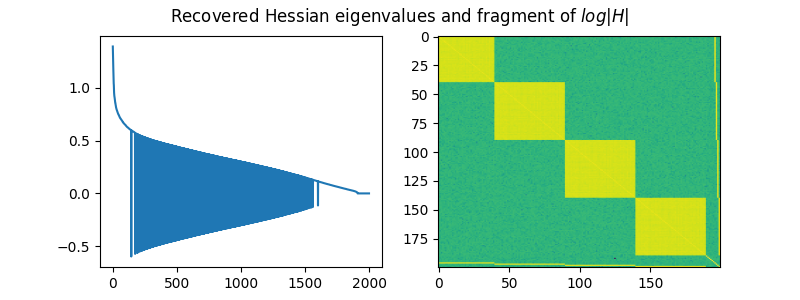
fig, (ax1, ax2) = plt.subplots(ncols=2, figsize=(8, 3))
ax1.plot(ews.cpu())
ax2.imshow(((evs[-200:] * ews) @ evs[-200:].T).abs().log().cpu(), aspect="auto")
fig.suptitle("Recovered Hessian eigenvalues and fragment of $log |H|$")

rel_err = (err_sq / frob_sq) ** 0.5
print("Estimated Hessian norm:", frob_sq.item() ** 0.5)
print("Estimated approximation error:", err_sq.item() ** 0.5)
print("RELATIVE ERROR:", (err_sq / frob_sq).item() ** 0.5)

Estimated Hessian norm: 16.62060580585183
Estimated approximation error: 6.613247817472402e-05
RELATIVE ERROR: 3.978945100209745e-06