Sketched Low-Rank Decompositions

In this example we create noisy, numerically low-rank matrices and compare their skerch low-rank SVD with the built-in torch counterparts (Full PyTorch SVD and Sketched PyTorch SVD) in terms of their scope, accuracy and speed, showing that skerch is superior.

Regarding scope, the key observation here is that skerch only requires a bare-minimum interface: compatible linear operators just have to provide a .shape = (height, width) attribute and implement the @ matmul operator from the left and right handside. Trying to run such a simple object using the torch alternatives listed above does not work, because they have more interface requirements.

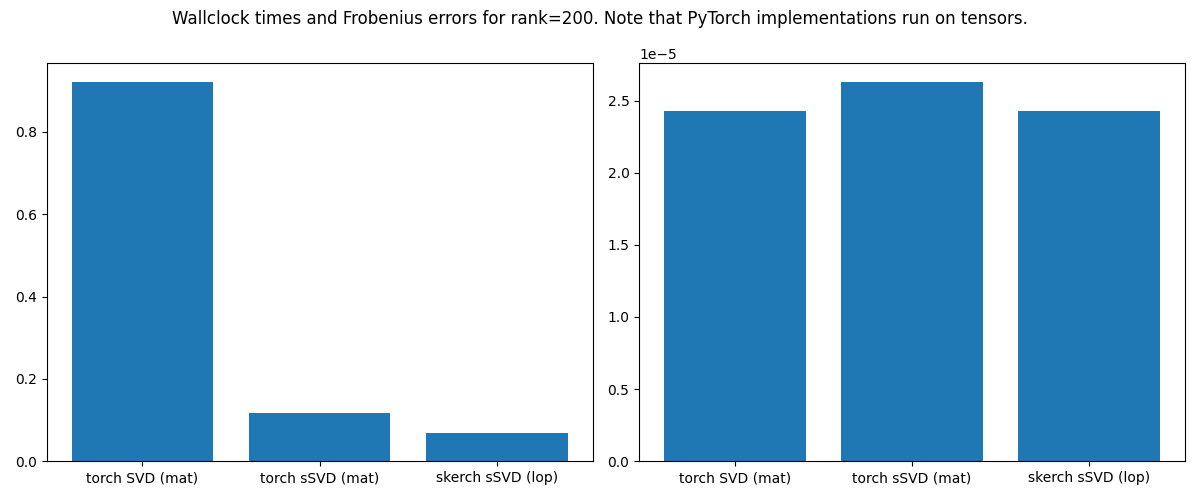
Regarding runtime and accuracy, we observe that skerch is competitive: the fact that we can flexibly choose noise source allows us to go for Rademacher, which yields same accuracy while being faster.

This showcases the main strength of skerch: we can fully leverage the flexibility and power of sketched methods without compromising scope, accuracy or speed (in Extending With Custom Functionality we also see how to easily add new noise sources and recovery methods into skerch).

Finally, we showcase the a-posteriori functionality, which also works on the bare-minimum interface and can be used to assess rank and quality of the recovery, even when the original matrix is still unknown or intractable.

from time import time

import matplotlib.pyplot as plt
import torch

from skerch.a_posteriori import apost_error, apost_error_bounds, scree_bounds
from skerch.algorithms import ssvd
from skerch.linops import CompositeLinOp, DiagonalLinOp
from skerch.synthmat import RandomLordMatrix
from skerch.utils import truncate_decomp

---

Creation of test data

We start by sampling an (approximately) low-rank matrix using skerch.synthmat.RandomLordMatrix. This is very convenient since it allows us fine control over the rank, spectral decay, symmetry and diagonal strength (see Synthetic Matrices).

Then we create a bare-bones linear operator from that matrix, to illustrate that most existing routines have more restrictive interfaces:

SEED = 54321
DEVICE = "cpu"
DTYPE = torch.complex64
SHAPE, RANK, DECAY = (1500, 1500), 100, 0.05
SKETCH_MEAS, TEST_MEAS = 200, 30


class MatLinOp:
    """Bare-bones linear operator, equivalent to the given matrix."""

    def __init__(self, matrix):
        self.matrix = matrix
        self.shape = matrix.shape

    def __matmul__(self, x):
        return self.matrix @ x

    def __rmatmul__(self, x):
        return x @ self.matrix


mat = RandomLordMatrix.exp(
    SHAPE, RANK, DECAY, symmetric=False, device=DEVICE, dtype=DTYPE, psd=False
)[0]
lop = MatLinOp(mat)

---

Compatibility with bare-bones linear operators

We now observe that both torch.linalg.svd and torch.svd_lowrank crash when we try to run them on our bare-bones linear operator:

try:
    _ = torch.linalg.svd(lop)
    raise RuntimeError("This should never happen!")
except TypeError as te:
    print("Expected torch.linalg.svd error on linop:", te)

try:
    _ = torch.svd_lowrank(lop)
    raise RuntimeError("This should never happen!")
except AttributeError as te:
    print("Expected torch.svd_lowrank error on linop:", te)

Expected torch.linalg.svd error on linop: linalg_svd(): argument 'A' (position 1) must be Tensor, not MatLinOp
Expected torch.svd_lowrank error on linop: 'MatLinOp' object has no attribute 'is_complex'

---

Sketched low-rank approximations

We now compute the in-core sketched SVD via skerch.algorithms.ssvd(). Since the torch alternatives don’t run on the bare-bones lop interface, we run them using the explicit mat. Note that, as already established, this is not a fair comparison in terms of scope, since skerch makes less assumptions about its input, but runtime and accuracy are still competitive:

t0 = time()
U1, S1, Vh1 = torch.linalg.svd(mat)
t1 = time() - t0
U1, S1, Vh1 = U1[:, :SKETCH_MEAS], S1[:SKETCH_MEAS], Vh1[:SKETCH_MEAS]
#
t0 = time()
U2, S2, Vh2 = torch.svd_lowrank(mat, q=SKETCH_MEAS, niter=1)
t2 = time() - t0
# Rademacher noise is faster and works as well as Gaussian.
# Note that we add one extra measurement, that we truncate later, for
# numerical stability
t0 = time()
U3, S3, Vh3 = ssvd(
    lop,  # runs on lop!
    DEVICE,
    DTYPE,
    SKETCH_MEAS + 1,
    seed=SEED,
    noise_type="rademacher",
    recovery_type="hmt",
)
U3, S3, Vh3 = truncate_decomp(SKETCH_MEAS, U3, S3, Vh3, copy=False)
t3 = time() - t0
times = (t1, t2, t3)

U3, S3, Vh3 = (
    U1[:, :SKETCH_MEAS],
    S1[:SKETCH_MEAS],
    Vh1[:SKETCH_MEAS],
)

matnorm = mat.norm()
err1 = torch.dist(mat, (U1 * S1) @ Vh1).item()
err2 = torch.dist(mat, (U2 * S2) @ Vh2.H).item()
err3 = torch.dist(mat, (U3 * S3) @ Vh3).item()

fig, (ax1, ax2) = plt.subplots(ncols=2, figsize=(12, 5))
ax1.bar(["torch SVD (mat)", "torch sSVD (mat)", "skerch sSVD (lop)"], times)
ax2.bar(
    ["torch SVD (mat)", "torch sSVD (mat)", "skerch sSVD (lop)"],
    (err1, err2, err3),
)
fig.suptitle(
    f"Wallclock times and Frobenius errors for rank={SKETCH_MEAS}. "
    "Note that PyTorch implementations run on tensors."
)
fig.tight_layout()

---

Approximate error analysis

In the code above, we used torch.dist to measure the error between original and recovery. This required us to express them as matrices.

When the linear operator is too large or matrix-free, which is the main point of skerch here, this kind of exact error analysis is not always possible, and we resort to approximate a posteriori methods (see skerch.a_posteriori for more details). Crucially, this also works on the bare-bones interface: we only require that the input components implement the .shape = (height, width) attribute and the @ matmul operator:

lop1 = CompositeLinOp([("U", U1), ("S", DiagonalLinOp(S1)), ("Vh_k", Vh1)])
lop2 = CompositeLinOp([("U", U2), ("S", DiagonalLinOp(S2)), ("Vh_k", Vh2.H)])
lop3 = CompositeLinOp([("U", U3), ("S", DiagonalLinOp(S3)), ("Vh_k", Vh3)])

(_, _, err1sq), _ = apost_error(
    mat, lop1, DEVICE, DTYPE, num_meas=TEST_MEAS, seed=SEED + max(SHAPE) * 2
)
(_, _, err2sq), _ = apost_error(
    mat, lop2, DEVICE, DTYPE, num_meas=TEST_MEAS, seed=SEED + max(SHAPE) * 2
)
(_, f3sq, err3sq), _ = apost_error(
    mat, lop3, DEVICE, DTYPE, num_meas=TEST_MEAS, seed=SEED + max(SHAPE) * 2
)


width = 0.2
fig, ax = plt.subplots(figsize=(8, 4))

# Bars for each tuple
ax.bar(torch.arange(3) - width / 2, (err1, err2, err3), width, label="Exact")
ax.bar(
    torch.arange(3) + width / 2,
    (err1sq.item() ** 0.5, err2sq.item() ** 0.5, err3sq.item() ** 0.5),
    width,
    label="Approximate",
)
ax.set_xticks(torch.arange(3))
ax.set_xticklabels(["torch SVD", "torch sSVD", "skerch sSVD"])
ax.legend()
fig.suptitle(
    f"Exact vs approximate error estimation for {TEST_MEAS} test measurements"
)
fig.tight_layout()

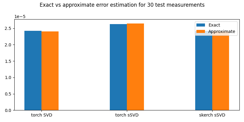
We see that the approximate errors are very close to the previously computed exact ones. The probability of this not happening, for any given number of a posteriori measurements and error tolerance (in this case 50%), can be obtained as follows (see also Command Line Interface):

apost_error_bounds(TEST_MEAS, 0.5)

{'LOWER: P(err<=0.5x)': 0.055177075636476565, 'HIGHER: P(err>=1.5x)': 0.24219226655288198}

---

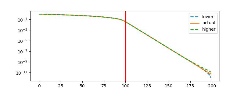
A posteriori rank estimation

We can also use the sketched decomposition and the a-posteriori computations to obtain the scree bounds plotted below. For each k (x-axis), the scree plot indicates the relative error of our sketched approximation, if it was truncated to rank-k.

These upper and lower bounds can be used to estimate the effective rank of the original operator, e.g. by looking for “elbows” in the scree curve. In this case, we have a simple synthetic matrix and a good sketched apporximation, so we can see how the scree bounds accurately and clearly reflect the given RANK of the original operator (signaled with a vertical line):

scree_lo, scree_hi = scree_bounds(S3, err3sq**0.5)
svals = torch.linalg.svdvals(mat)
scree_true = (svals**2).flip(0).cumsum(0).flip(0)[: len(S3)] / (svals**2).sum()

fig, ax = plt.subplots(figsize=(8, 3))
ax.plot(scree_lo.cpu(), label="lower", ls="--", linewidth=2)
ax.plot(scree_true.cpu(), label="actual", linewidth=2)
ax.plot(scree_hi.cpu(), label="higher", ls="--", linewidth=2)
ax.axvline(RANK, color="red", linewidth=2)
ax.set_yscale("log")
ax.legend()

<matplotlib.legend.Legend object at 0x71385f19acb0>

---

And we are done!

• We have seen how to perform sketched SVDs with skerch on linear operators that support a bare-minimum interface. This is not directly possible with other torch implementations

• We observed that the skerch implementation has bare-minimum requirements on the interface of the linear operators provided, working where other implementations don’t, with competitive runtime and accuracy

• We also demonstrated matrix-free, scalable methods to verify the quality of the sketched approximation and to estimate the rank of the original operator