Traces, Diagonals, Triangles

In this example we explore the following skerch functionality:

• Trace and diagonal estimations

• Triangular matrix-vector multiplications

Given a linear operator \(A\), we first perform stochastic trace and diagonal estimation using XDiag/Huch++ (see skerch.algorithms.xhutchpp()). Computations needed for both estimations are very similar and can be mostly recycled to compute both quantities at once. To illustrate the effect of low-rank deflation, we run these methods on a full-rank and a low-rank matrix.

Then, we move onto triangular mat-vec estimation, i.e. \(tril(A) v\) and \(triu(A) v\), which also makes use of a modification of Girard-Hutchinson combined with deterministic measurements.

We verify the accuracy of the sketched approximations by comparing them to the actual quantities.

Note

One core feature of Girard-Hutchinson is its rather slow convergence rate: in general, doing just a few noisy measurements can introduce large amounts of error and be worse that not doing it at all (especially if entries in the measurement vectors span multiple orders of magnitude). If the diagonal is not very prominent and the operator has a flat spectrum, measurements needed for a reliable estimate must be typically in the order of thousands (see Table 1 in [BN2022] for bounds).

import matplotlib.pyplot as plt
import torch

from skerch.algorithms import TriangularLinOp, xhutchpp
from skerch.synthmat import RandomLordMatrix
from skerch.utils import gaussian_noise

---

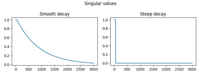
Creation of test matrices

We create two matrices, with smooth and fast decaying spectrum:

SEED = 392781
DEVICE = "cuda" if torch.cuda.is_available() else "cpu"
DTYPE = torch.float64
DIMS, RANK = 3000, 50
DEFL_DIMS, GH_MEAS = 80, 1500

shape = (DIMS, DIMS)
mat = RandomLordMatrix.exp(
    shape, RANK, 0.0005, seed=SEED + 1, device=DEVICE, dtype=DTYPE
)[0]
lomat = RandomLordMatrix.exp(
    shape, RANK, 0.5, seed=SEED, device=DEVICE, dtype=DTYPE
)[0]

fig, (ax1, ax2) = plt.subplots(ncols=2, figsize=(8, 3))
ax1.plot(torch.linalg.svdvals(mat.cpu()))
ax2.plot(torch.linalg.svdvals(lomat.cpu()))
ax1.set_title("Smooth decay")
ax2.set_title("Steep decay")
fig.suptitle("Singular values")
fig.tight_layout()

---

Trace and diagonal estimation via XHutch++

XHutch++ (see skerch.algorithms.xhutchpp()) immplements both XDiag and plain Girard-Hutchinson to estimate the trace and/or the diagonal. XDiag is generally the preferred choice (unless our matrix has a very flat spectrum), but it has one drawback: It requires us to store as many vectors as measurements, which may not always be possible. With xhutchpp we can set DEFL_DIMS to whatever we can afford in terms of memory, and then independently set GH_MEAS to perform further measurements on top, at no substantial overhaead in memory:

hutch1 = xhutchpp(
    mat,
    DEVICE,
    DTYPE,
    DEFL_DIMS,
    GH_MEAS,
    seed=SEED + 2 * DIMS,
    noise_type="rademacher",
    meas_blocksize=None,
    return_diag=True,
)

hutch2 = xhutchpp(
    lomat,
    DEVICE,
    DTYPE,
    DEFL_DIMS,
    GH_MEAS,
    seed=SEED + 3 * DIMS,
    noise_type="rademacher",
    meas_blocksize=None,
    return_diag=True,
)

tr1, diag1 = hutch1["tr"], hutch1["diag"]
tr2, diag2 = hutch2["tr"], hutch2["diag"]

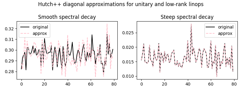
We now assess output quality by visually inspecting the diagonals and measuring relative errors, observing that both are well below 5%:

def relerr(ori, rec, squared=True):
    """Relative error in the form ``(frob(ori - rec) / frob(ori))**2``."""
    result = (ori - rec).norm() / ori.norm()
    if squared:
        result = result**2
    return result


def relsumerr(ori_sum, rec_sum, ori_vec, squared=True):
    """Relative error of a sum of estimators.

    The error for adding N estimators is bounded by ``sqrt(N)`` times the
    norm of said estimators, because:
    ``(1^T ori) - (1^T rec) = 1^T (ori - rec)``, and the norm of this, by
    Applying Cauchy-Schwarz:
    ``norm(1^T (ori - rec)) <= norm(1)*norm(ori-rec) = sqrt(N)*norm(ori-rec)``.

    So, for the sum of entries, we apply ``relerr``, but divided by ``sqrt(N)``
    to account for this factor:

    ``| ori_sum - rec_sum |`` / (sqrt(N) * norm(ori_vec))``.

    This is consistent in the sense that, if rec_vec is close to ori_vec by
    0.001, this metric will also output at most 0.001 for the estimated sum.
    """
    result = abs(ori_sum - rec_sum) / (len(ori_vec) ** 0.5 * ori_vec.norm())
    if squared:
        result = result**2
    return result


# ground-truth values
mat_diag, lomat_diag = mat.diag(), lomat.diag()
mat_tr, lomat_tr = mat_diag.sum(), lomat_diag.sum()
# relative errors
tr1_err = relsumerr(mat_tr, tr1, mat_diag, squared=False).item()
tr2_err = relsumerr(lomat_tr, tr2, lomat_diag, squared=False).item()
diag1_err = relerr(mat_diag, diag1, squared=False).item()
diag2_err = relerr(lomat_diag, diag2, squared=False).item()

beg, end = 0, 80
fig, (ax1, ax2) = plt.subplots(ncols=2, figsize=(8, 3))
ax1.plot(mat_diag[beg:end].cpu(), color="black", label="original")
ax1.plot(diag1[beg:end].cpu(), color="pink", linestyle="--", label="approx")
ax1.set_title("Smooth spectral decay")
ax1.legend()
ax2.plot(lomat_diag[beg:end].cpu(), color="black", label="original")
ax2.plot(diag2[beg:end].cpu(), color="pink", linestyle="--", label="approx")
ax2.legend()
ax2.set_title("Steep spectral decay")
fig.suptitle("Hutch++ diagonal approximations for unitary and low-rank linops")
fig.tight_layout()

print("Trace relative error (smooth):", tr1_err)
print("Trace relative error (steep):", tr2_err)
print("Diagonal relative error (smooth):", diag1_err)
print("Diagonal relative error (steep):", diag2_err)

Trace relative error (smooth): 0.00031970191355760834
Trace relative error (steep): 1.381857308138173e-16
Diagonal relative error (smooth): 0.021938503124878654
Diagonal relative error (steep): 2.434902156443878e-15

---

Triangular matrix-vector estimation

Similar in spirit to skerch.algorithms.xhutchpp(), skerch.algorithms.TriangularLinOp wraps any given linear operator (as long as it implements the .shape = (height, width) attribute and the @ matmul operation), and combines deterministic staircase-shaped measurements with a modification of Girard-Hutchinson in order to estimate triangular matrix-vector products in the form tri(lop) @ v. Here we can also customize many aspects, including how many measurements are performed in each part:

ltri = TriangularLinOp(
    mat,
    stair_width=max(1, DIMS // 20),
    num_gh_meas=GH_MEAS,
    lower=True,
    with_main_diagonal=False,
    seed=SEED + 4 * DIMS,
    noise_type="rademacher",
)

# ground truth values for triangular matrix product
v = gaussian_noise(DIMS, 0, 1, seed=SEED - 1, dtype=DTYPE, device=DEVICE)
mat_tril = mat.tril(-1)
w1 = mat_tril @ v
w2 = v @ mat_tril

# sketched approximations
ltri_w1 = ltri @ v
ltri_w2 = v @ ltri

# relative errors
w1_err = relerr(w1, ltri_w1, squared=False).item()
w2_err = relerr(w2, ltri_w2, squared=False).item()


beg, end = 0, 100
fig, (ax1, ax2) = plt.subplots(ncols=2, figsize=(8, 3))
ax1.plot(w1[beg:end].cpu(), color="black", label="original")
ax1.plot(ltri_w1[beg:end].cpu(), color="pink", linestyle="--", label="approx")
ax1.set_title("$tril(A) v$")
ax1.legend()
ax2.plot(w2[beg:end].cpu(), color="black", label="original")
ax2.plot(ltri_w2[beg:end].cpu(), color="pink", linestyle="--", label="approx")
ax2.set_title("$v^T tril(A) $")
ax2.legend()
fig.tight_layout()


print("Lower-triangular relative error:", w1_err)
print("Lower-triangular relative error (adjoint):", w2_err)

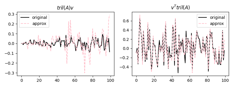
Lower-triangular relative error: 0.47159650162777184
Lower-triangular relative error (adjoint): 0.46202995254752677

---

And we are done!

• We have seen how to estimate traces, diagonals and triangular matrix multiplications using skerch, and only requiring the bare-minimum interface for linear operators

• We illustrated the effectiveness of low-rank deflation as well as the tendency of Girard-Hutchinson to need more measurements