Synthetic Matrices

Many sketched algorithms are made to work on specific types of operators, such as low-rank or diagonally dominant. Typically, we want to test such algorithms on operators that satisfy these properties to a given extent (e.g. random matrices with a spectrum that decays in a specific way).

In this example, we explore the functionality in skerch.synthmat, which allows us to generate a broad class of synthetic matrices with desired properties. Specifically:

• Random (approximately) low-rank plus diagonal matrices

import matplotlib.pyplot as plt
import torch

from skerch.synthmat import RandomLordMatrix

---

Low-rank plus diagonal (LoRD) matrices

The skerch.synthmat.RandomLordMatrix class allows to generate matrices in the form \(L + \alpha D\), where \(D\) is diagonal and \(L\) is approximately low-rank,has RANK singular values fixed to 1, followed by a configurable spectral decay. The \(\alpha\) scalar (in the code: diag_ratio) represents the diagonal dominance of the matrix: the larger, the closer to a diagonal.

SEED = 1337
DEVICE = "cuda" if torch.cuda.is_available() else "cpu"
DTYPE = torch.float32
DIMS, RANK = 20, 5
SV_DECAYS, DIAG_RATIOS = (0.5, 0.1, 0.01), (0, 1, 10)

matrices = {}
svals = {}
for exp_decay in SV_DECAYS:
    for diag_ratio in DIAG_RATIOS:
        mat = RandomLordMatrix.exp(
            (DIMS, DIMS),
            RANK,
            exp_decay,
            diag_ratio=diag_ratio,
            symmetric=False,
            device=DEVICE,
            dtype=DTYPE,
        )[0]
        sv = torch.linalg.svdvals(mat)
        matrices[(exp_decay, diag_ratio)] = mat
        svals[(exp_decay, diag_ratio)] = sv

Let’s plot the matrices and their singular values to get a better picture!

def plot_matrix(ax, mat, cmap="seismic", aspect="auto", dampen=4.0):
    lo, hi = mat.min(), mat.max()
    maxabs = max(abs(lo), abs(hi)) * dampen
    ax.imshow(mat, cmap=cmap, vmin=-maxabs, vmax=maxabs, aspect=aspect)


def plot_svals(ax, svals):
    dims = len(svals)
    min_sv, max_sv = svals.min(), svals.max()
    sv_norm = (svals - min_sv) / (max_sv - min_sv)  # from 0 to 1
    sv_scaled = 1 * (dims - 1) * (1 - sv_norm)
    ax.plot(
        range(dims), sv_scaled, c="k", marker="o", markersize=4, linewidth=1.5
    )


fig, axs = plt.subplots(nrows=len(DIAG_RATIOS), ncols=len(SV_DECAYS))
for i, diag_ratio in enumerate(DIAG_RATIOS):
    for j, exp_decay in enumerate(SV_DECAYS):
        plot_matrix(axs[i, j], matrices[(exp_decay, diag_ratio)].cpu())
        plot_svals(axs[i, j], svals[(exp_decay, diag_ratio)].cpu())
        axs[i, j].set_xticks([])
        axs[i, j].set_yticks([])

for i, diag_ratio in enumerate(DIAG_RATIOS):
    axs[i, 0].set_ylabel(f"diag ratio={diag_ratio}")
for i, exp_decay in enumerate(SV_DECAYS):
    axs[-1, i].set_xlabel(f"exp decay={exp_decay}")

fig.suptitle("Sampled LoRD matrices, with singular values plotted on top")
fig.tight_layout()

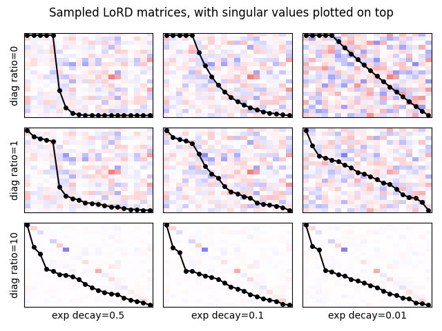
We see now how increasing diag_ratio makes the diagonal more prominent and at the same time leaks into the singular values, making the matrix less low-rank. We also see that the exp_decay ratio also determines how quickly do the singular values decay after RANK.