Linear Operators and Matrix-Freedom

In this example we explore some of the functionality from the skerch linear operator API, specifically:

• Creation of a skerch-compatible linear operator (bare-minimum interface)

• Matrix-free transposition

• Wrapping NumPy-only linear operators into PyTorch

• Composition and addition of linear operators

• Matrix-free diagonal linear operators

• Matrix-free noisy linear operators for sketching

This functionality allows us to perform sketches and work with linear operators at scale.

from time import time

import matplotlib.pyplot as plt
import torch

from skerch.algorithms import snorm
from skerch.linops import (
    CompositeLinOp,
    DiagonalLinOp,
    TorchLinOpWrapper,
    TransposedLinOp,
    linop_to_matrix,
)
from skerch.measurements import (
    GaussianNoiseLinOp,
    PhaseNoiseLinOp,
    RademacherNoiseLinOp,
    SsrftNoiseLinOp,
)
from skerch.utils import gaussian_noise

---

Creating a skerch-compatible linop

To work with skerch, linear operators must satisfy only 2 requirements, resulting in a bare-minimum linop interface:

• They must support left- and right-matrix multiplication via @

• They must feature a .shape = (height, width) attribute

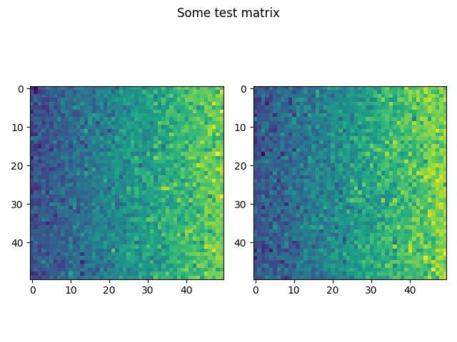
This is satisfied by regular matrices like the following mat:

SHAPE = (50, 50)
NUM_MEAS = 10
SEED = 12345
DTYPE = torch.complex64
DEVICE = "cuda" if torch.cuda.is_available() else "cpu"

mat = gaussian_noise(SHAPE, 0, 10, seed=SEED, dtype=DTYPE, device=DEVICE)
ramp = torch.arange(mat.shape[1], dtype=mat.real.dtype, device=mat.device)
mat += ramp + 1j * ramp

fig, (ax1, ax2) = plt.subplots(ncols=2)
ax1.imshow(mat.real.cpu())
ax2.imshow(mat.imag.cpu())
fig.suptitle("Some test matrix")
fig.tight_layout()

But matrices also allow for other operations such as arbitrary indexing like mat[5, 7]. This is something that many linear operators don’t or cannot provide without substantial overhead.

In those restricted cases, we are dealing with a matrix-free linear operator, of potentially very large scale, defined mainly by its dimensions and matmul functionality.

As an example, the following linop implements the bare-minimum interface. We see that, despite this limitation, we can successfully apply skerch.algorithms.snorm() to estimate its operator norm:

class SomeLinOp:
    """Some matrix-free linop to exemplify skerch-compatibility."""

    def __init__(self, dims):
        self.shape = (dims, dims)

    def __matmul__(self, x):
        result = x * 0.5
        result[0, ...] += x.sum(dim=0)
        return result

    def __rmatmul__(self, x):
        result = x * 0.5
        result = (result.transpose(0, -1) + x[..., 0]).transpose(0, -1)
        return result


lop = SomeLinOp(SHAPE[0])
lopmat = linop_to_matrix(lop, dtype=ramp.dtype, device="cpu")
lop_S = torch.linalg.svdvals(lopmat)
op_norm = snorm(
    lop,
    DEVICE,
    DTYPE,
    num_meas=NUM_MEAS,
    seed=SEED + 123,
    noise_type="gaussian",
    norm_types=["op"],
)[0]["op"]
print("Actual norm:", torch.linalg.svdvals(lopmat).max().item())
print("Sketched norm:", op_norm.item())

fig, ax = plt.subplots(figsize=(8, 4))
ax.imshow(lopmat)
fig.suptitle("The linear operator, in matrix form")
fig.tight_layout()

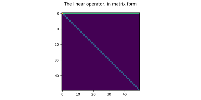
Actual norm: 7.175588607788086
Sketched norm: 7.088768482208252

---

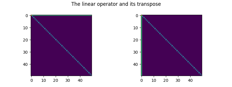
Matrix-free transposition

We can also use skerch.linops.TransposedLinOp to transpose linear operators in a matrix-free fashion:

lopT = TransposedLinOp(lop)

fig, (ax1, ax2) = plt.subplots(ncols=2, figsize=(8, 3))
ax1.imshow(linop_to_matrix(lop, dtype=ramp.dtype, device="cpu"))
ax2.imshow(linop_to_matrix(lopT, dtype=ramp.dtype, device="cpu"))
fig.suptitle("The linear operator and its transpose")
fig.tight_layout()

---

PyTorch wrapper

Since skerch is built on PyTorch, it won’t directly work on numpy linops that don’t accept PyTorch inputs. This can be solved with the wrapper, which also tracks the torch.device:

class NumpyFlipLinOp:
    """Numpy-only antidiagonal linop. Doesn't work with torch tensors."""

    def __init__(self, shape):
        self.shape = shape

    def __matmul__(self, x):
        return x[::-1].copy()

    def __rmatmul__(self, x):
        return self.__matmul__(x)


class TorchFlipLinOp(TorchLinOpWrapper, NumpyFlipLinOp):
    """This wrapper works with tensors and numpy arrays."""


np_lop = NumpyFlipLinOp(SHAPE)
torch_lop = TorchFlipLinOp(SHAPE)
arr = ramp.cpu().numpy()


print("Numpy linop on numpy data:", np_lop @ arr)
print("Wrapped linop on numpy data:", torch_lop @ arr)
print("Wrapped linop on torch data:", torch_lop @ ramp)

Numpy linop on numpy data: [49. 48. 47. 46. 45. 44. 43. 42. 41. 40. 39. 38. 37. 36. 35. 34. 33. 32.
 31. 30. 29. 28. 27. 26. 25. 24. 23. 22. 21. 20. 19. 18. 17. 16. 15. 14.
 13. 12. 11. 10.  9.  8.  7.  6.  5.  4.  3.  2.  1.  0.]
Wrapped linop on numpy data: [49. 48. 47. 46. 45. 44. 43. 42. 41. 40. 39. 38. 37. 36. 35. 34. 33. 32.
 31. 30. 29. 28. 27. 26. 25. 24. 23. 22. 21. 20. 19. 18. 17. 16. 15. 14.
 13. 12. 11. 10.  9.  8.  7.  6.  5.  4.  3.  2.  1.  0.]
Wrapped linop on torch data: tensor([49., 48., 47., 46., 45., 44., 43., 42., 41., 40., 39., 38., 37., 36.,
        35., 34., 33., 32., 31., 30., 29., 28., 27., 26., 25., 24., 23., 22.,
        21., 20., 19., 18., 17., 16., 15., 14., 13., 12., 11., 10.,  9.,  8.,
         7.,  6.,  5.,  4.,  3.,  2.,  1.,  0.])

---

Other linear operators

We can perform matrix-free compositions and additions of linear operators. Other matrix-free structured linops, such as diagonal and banded, are also available (see skerch.linops). Here we exemplify composition:

k = 2
U, S, Vh = torch.linalg.svd(mat.cpu())

lop_k = CompositeLinOp(
    [("U_k", U[:, :k]), ("S_k", DiagonalLinOp(S[:k])), ("Vh_k", Vh[:k, :])]
)

fig, (ax1, ax2) = plt.subplots(ncols=2, figsize=(8, 3))
ax1.imshow(mat.real.cpu())
ax2.imshow(linop_to_matrix(lop_k, dtype=mat.dtype, device="cpu").real)
fig.suptitle(f"Matrix and its rank-{k} matrix-free approximation [{lop_k}]")
fig.tight_layout()

---

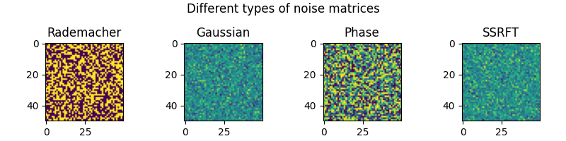
Matrix-free noisy linear operators for sketching

In order to run the sketches, skerch provides built-in support for noisy measurements in the form of matrix-free linear operators. In order to facilitate parallelized measurements, these linops have a bit more restrictive requirements than the bare-minimum interface discussed above: Besides the .shape and @ properties required by all skerch linops, they also must also implement a get_blocks iterator, that yields blocks of columns with their indices.

A good way to satisfy this interface and add a new noise type to skerch is to extend skerch.linops.ByBlockLinOp with get_block (see Extending With Custom Functionality for an example).

The figure below illustrates some of the already supported types of noise:

blocksize = 5
mop1 = RademacherNoiseLinOp(SHAPE, SEED, blocksize=blocksize)
mop2 = GaussianNoiseLinOp(SHAPE, SEED, blocksize=blocksize)
mop3 = PhaseNoiseLinOp(SHAPE, SEED, blocksize=blocksize)
mop4 = SsrftNoiseLinOp(SHAPE, SEED, blocksize=blocksize)

fig, (ax1, ax2, ax3, ax4) = plt.subplots(ncols=4, figsize=(8, 2))
ax1.imshow(mop1.to_matrix(DTYPE, "cpu").real)
ax2.imshow(mop2.to_matrix(DTYPE, "cpu").real)
ax3.imshow(mop3.to_matrix(DTYPE, "cpu").real)
ax4.imshow(mop4.to_matrix(DTYPE, "cpu").real)
#
ax1.set_title("Rademacher")
ax2.set_title("Gaussian")
ax3.set_title("Phase")
ax4.set_title("SSRFT")
fig.suptitle("Different types of noise matrices")
fig.tight_layout()

And the line below illustrates the behaviour of get_blocks:

[(b.shape, idxs) for b, idxs in mop1.get_blocks(DTYPE)]

[(torch.Size([50, 5]), range(0, 5)), (torch.Size([50, 5]), range(5, 10)), (torch.Size([50, 5]), range(10, 15)), (torch.Size([50, 5]), range(15, 20)), (torch.Size([50, 5]), range(20, 25)), (torch.Size([50, 5]), range(25, 30)), (torch.Size([50, 5]), range(30, 35)), (torch.Size([50, 5]), range(35, 40)), (torch.Size([50, 5]), range(40, 45)), (torch.Size([50, 5]), range(45, 50))]

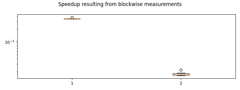
To illustrate the necessity of blockwise measurements, consider the following example, where a larger block size results in substantially faster computations:

mop_shape = (mat.shape[1], 100)
mop_slow = RademacherNoiseLinOp(mop_shape, SEED, blocksize=1, register=False)
mop_fast = RademacherNoiseLinOp(mop_shape, SEED, blocksize=100, register=False)
times = [[], []]
for _ in range(20):
    t0 = time()
    mat @ mop_slow
    times[0].append(time() - t0)
    #
    t0 = time()
    mat @ mop_fast
    times[1].append(time() - t0)

fig, ax = plt.subplots(figsize=(8, 3))
ax.boxplot(times, label=["blocksize=1", "blocksize=100"])
ax.set_yscale("log")
fig.suptitle("Speedup resulting from blockwise measurements")
fig.tight_layout()

---

This concludes the skerch tour of linear operators! Please refer to the API docs and other examples. for more details. In summary:

• We have seen how to create simple matrix-free linops, so that they are compatible with the skerch routines

• We also saw how to manipulate said linops, by transposing them, converting them to matrices and wrapping them to ensure NumPy compatibility in-core sketched methods for a broad class of low-rank matrices

• We explored other available linear operators, including compositions and noisy measurement linops, emphasizing the benefit of blockwise measurements